This post discusses one of the essential ingredients for training a model: how to see whether your model is actually improving, in other words, how do you benchmark the result of your training? Please read our prior blog posts (e.g. On incentive (part 1)) to understand the concept of sample loss values and the loss being used as a proxy for model quality.
Where to start?
In the bittensor eco-system in general, and our subnet in particular, distributed and collaborative effort is one of the corner stones. For model training, it means you typically start from a pre-existing model. Indeed, beginning from scratch is a non-starter, since it will require many thousands of GPU-hours before a brand-new model is on-par with an existing one, with which you usually have to compete. In SN29, we do have separate competitions for different model types, but not for different model sizes, as we feel/know you can always convert a small model to a bigger one by adding layers or increasing intermediate state-size. Also, larger models should only be valuable if they beat smaller models anyway, otherwise they are mostly useless. We believe in incremental progress, also by growing smaller models progressively into larger ones.
After choosing a model, start training!
So, you take an existing model and start training using your favorite optimizer, learning rate and all other hyper-parameters you can think of. How do you assess whether your efforts are working out? The simplest way is to just observe the average loss during the training. The loss values seen during training are the by-product of the training process, and by collecting these loss values you can get an indication of the state of the model, for example by averaging them and (hopefully) seeing the average loss go down. If a model is not trained very well yet, this is an easy approach and will be helpful to monitor progress. But later on, you’ll notice that this signal is noisy, and it starts to look saturated.
Noisy signal?
Each sample is unique and has its own loss value, that depends both on the model and on the sample. Just looking at a single loss value doesn’t tell you much. If you look at a collection of loss values you will quickly see that there is significant variation: we see this variation as noise in the signal that we are observing. As the improvements get smaller, they are overwhelmed by the noise and it starts to look like progress is stalled. But is it, and should you indeed stop training? In our subnet, the advantage a model gets, decays exponentially, with an initial value of 0.4% and a halving time of about a week. This means that after two weeks, a loss improvement of 0.1% is enough to start winning. So it is still worth training if you can improve a model by 0.1%, but measuring such small improvements is not trivial.
Error bars
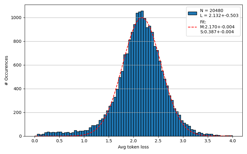
Because the average-loss-during-training-signal is so noisy, it is better to take a different metric. The scientific approach is to estimate and then reduce the error in the signal, that is, estimate the error bar. We normally use a reference dataset of 20480 randomly selected samples, which, in our training, is guaranteed to not overlap with the training dataset. If you don’t do this, you might be misled because obviously your trained model will score better on a sample it has seen before. You can also take a random set, as the fineweb-2 dataset is large and random selections of samples will not overlap often. If we compute the (per-token) losses on our reference dataset, we get the following distribution of losses:

This plot visualizes the points made above: while the average loss is ~2.17, the standard deviation (i.e. noise) is ~0.39!
Not normal
It is clear that this is not quite a normal distribution, but has some tail on the low-loss side. Some samples are very easy to predict, apparently, so probably memorized quite literally, leading to some low loss values. We did fit a gaussian here, as if it were a normal distribution, and the uncertainty in the fit gives an error bar for the average loss of about 0.18% (0.004/2.170). This is not just due to the non-gaussianity, but also due to the (fundamental, intrinsic) noise on the histogram bars.
Generalizing this analysis
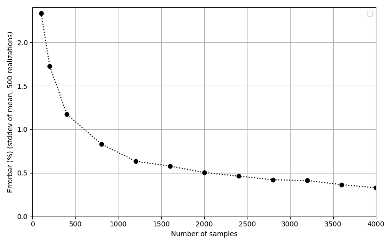
Using this big set we can try to answer questions about the error bar on the average loss, based on a smaller sample set. We do this by sampling a certain number of loss values from the above set and computing the average. If we repeat this procedure N times and determine the standard deviation of these N averages, we get an estimate of the error bar:

This graph tells us we need about 2000 samples to get an error bar of ~0.5%.
Not enough
From the above it is clear that as improvements get down to the 0.1% range, the error in the average-loss-during-training-signal is still too large to make a good judgement whether the model is even improving, and you may be wasting GPU hours on training with the wrong hyperparameters. You need something better to compare the trained model to the starting point.
Comparing models
It is straightforward to compare models on the same reference dataset. During the training process we benchmark the model-in-training on our reference dataset regularly. This way, we can detect a change in loss of order 0.001%. i.e. quite a bit smaller than the error bar according to the fit in graph 1! The reason is that we now know the exact shape of the distribution, instead of the assumption that it approximates a gaussian as if it were a normal distribution. Of course this does not guarantee that the model will perform better on any particular sample or set of samples, because the coverage may be limited. However, if the set is large enough it is a reasonable metric, and allows you to tweak your hyperparameters accordingly (a bit of an art) and assess the impact.
If we would try to compare different models based on their average loss on different samples though, which is what we would naively do if we monitor the loss values obtained as part of the training process, we are pretty much limited by the error bar of the fit in graph 1, i.e. approximately a factor 180 less sensitive… That’s the reason it’s so hard to determine whether the loss-during-training is still going down!
0 Comments