In this post, we revisit model comparison metrics. Should we compare sample-by-sample, or group several samples together? Or does it make more sense to “pack” samples (i.e. join multiple samples with an EOS token in between)? Does length matter? And what’s up with these “pages” in the dataset?
TL;DR
A minor modification to the incentive mechanism eliminates some systematic biases introduced by the structure of the validation dataset. This will lead to a better assessment of overall model quality and eliminate possible meta-gaming tactics. Broad training is further incentivized.
Sample losses
Let’s start with a plot of relative sample losses for two different models that score roughly equal on average:
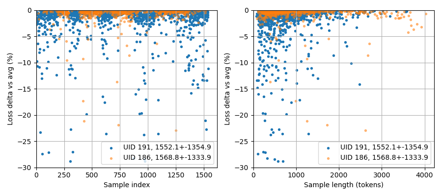
We are looking at the losses of two models in the Phi (c01) competition on SN29. On the left you see the relative difference between the two models (only the winning sample is plotted, so only values below 0%). There is a clear structure in this data, with some parts where the blue model is obviously much better, and others where the orange model wins. This structure originates in the way the data is fetched: in so-called pages from the fineweb-edu2 dataset. Each page contains 100 rows, and it looks like either their content is correlated in some way, and/or that models are trained better on some pages than on other pages; both of these options might explain how a model scoring well on one sample, scores well on other samples of that page.
On the right, you see a scatter of the relative scores of the two models versus the sample length in tokens. Here it is clear that the blue model wins often on the shorter samples, while the orange model might have a slight edge on longer samples.
Pages, pages and more pages
The fineweb dataset is huge, with roughly 5.9B rows of data. It is divided into several subsets, through which you can browse on huggingface. Here’s a screenshot of the CC-MAIN-2015-35 subset:
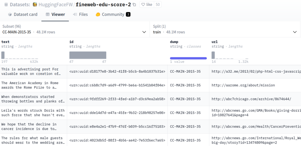
The data loader in the validator picks a number of pages (i.e. dataset + offset) and fetches 100 consecutive rows from each page it selected. As can be seen in the image above, these rows are possibly quite correlated. For starters, they are all from the same time period. In this case, that could mean the sentence “In the year…” is more likely to be followed by “2015” than any other year. Also, they are apparently sorted by url, and several rows can come from the same source, such as abcnews.go.com in this screenshot. It is to be expected that the contents of these rows are somewhat correlated.
We think it is this correlation that is visible in the plot of sample losses, shown above.
What to reward?
Up to now, scoring in SN29 was done by comparing loss values on a sample-by-sample basis. We see that this results in a relatively broad selection of models that gets rewarded. However, in the current setup, models are only rewarded for good sample scores, and not penalized for bad sample scores. We think this may lead to underperforming models being rewarded. For example, a model could be (over-)trained on content of the year 2015. It that case, it will score well on pages from a 2015 dataset, and worse on others. This means that it could be completely ignorant on anything about 2016 and later – but still win on some samples and get rewarded. Another bisection could be short and long samples, or any other feature (e.g. samples starting with a-m).
We want to reward models that score well across a wide range of samples. We could of course look at just the summed total sample loss, but it would make a fine-grained comparison between several different models tricky. An alternative is to sum smaller groups of samples, which we simulated to get a good estimate of the effect:
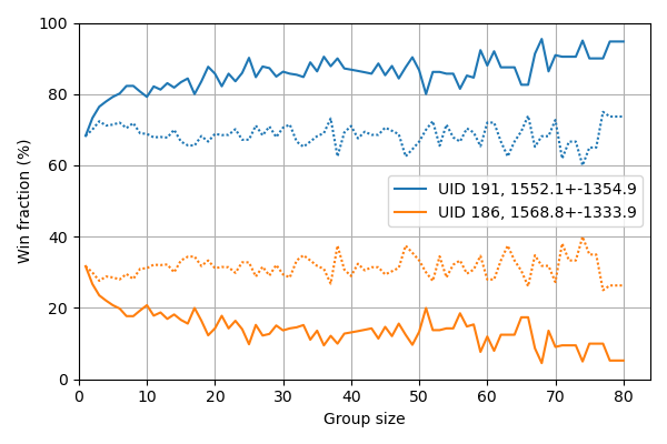
Here we take a number of samples (“group size”, on the x axis), and sum their loss to get the performance on a “super-sample”. We plot the win fraction versus super-sample group size for either consecutive samples (mostly from the same page, dotted line), or we shuffle before grouping (solid line). In the limit of a super-sample containing all samples, this metric is identical to comparing the average sample loss, and will result in a single 100% win.
It is clear that without shuffling the super-sample strategy does not make much of a difference and models could still be specialized to content present in a single page from the dataset, for example to a subset of websites, and earn reward for that. Therefore, we choose the new scoring mechanism to take random samples for the super-sample, so that we get a better estimate of the average performance. Effectively, this means that models will be penalized for scoring badly on some samples.
Comparison to packed samples
The super-sample strategy is somewhat similar to using “packed” samples. When packing samples, consecutive samples are concatenated with EOS tokens in between, until they reach some fixed number of tokens. This is particularly convenient for training, where equal-length token sequences can speed up the training process. However, in evaluation it is a weird thing: a model’s prediction of tokens following EOS is scored, which stands for End Of Stream, so it doesn’t make sense. Additionally, the packed samples may or may not be correlated, both cases influencing the sample score in weird ways. All this adds unwanted noise to the evaluation of a model’s performance, and introduces meta-gaming tactics that distract from the subnet goal.
Super-samples bring the benefits of sample-packing for evaluation – more tokens – but exclude the correlation issues. What remains is to determine a suitable grouping size. Below is a histogram of super-sample token length for several grouping sizes, taken from a shuffled set of 20k samples:
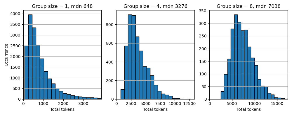
Subnet 29 will initially switch to a group size of 5, for a median super-sample length of 4200 tokens (as measured using the stock Phi tokenizer). We are convinced this will lead to a more balanced comparison between the submitted models and will subsequently incentivize broader training.
New metagaming tactics?
Sample grouping introduces a new metagaming tactic. To understand this, you need to first consider what happens if a sample has to be discarded because it is too long, that is, if its tokenized representation exceeds the maximum sequence length: The model will score Inf and that sample is lost compared to models that did get a score on the sample (which is possible because a model can have a different tokenizer). When grouping samples, the whole group is lost, which amplifies the effect. Suppose 2% of samples is discarded, after grouping with a group size of 5, approximately 10% of groups is discarded.
The metagaming tactic is then to create a model with an extremely efficient tokenizer, that is, with maybe ten times the normal amount of tokens. The sequence length for this model, will be significantly shorter than normally, and this model will get a score, where other models score Inf. Now this model will win those (groups of) samples, irrespective of the actual performance. If this would win the model 10% of groups, it is significant enough to gain some incentive. By truncating samples, before tokenization, to a length that is reasonable, this tactic is rendered ineffective.
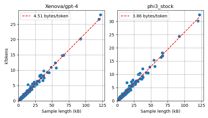
For a combination of a tokenizer and a dataset an average number of bytes per token can be derived, which can be used to calculate an approximate sample length for the maximum sequence length. This is implemented in the latest validator release.
0 Comments